Data Acquisition with APIs in R

You can download this .qmd file from here. Just hit the Download Raw File button.

Credit to Brianna Heggeseth and Leslie Myint from Macalester College for a few of these descriptions and examples.

Introduction to APIs

When we interact with sites like The New York Times, Zillow, and Google, we are accessing their data via a graphical layout (e.g., images, colors, columns) that is easy for humans to read but hard for computers.

An API stands for Application Programming Interface, and this term describes a general class of tool that allows computers, rather than humans, to interact with an organization’s data. How does this work?

When we use web browsers to navigate the web, our browsers communicate with web servers using a technology called HTTP or Hypertext Transfer Protocol to get information that is formatted into the display of a web page.
Programming languages such as R can also use HTTP to communicate with web servers. The easiest way to do this is via Web APIs, or Web Application Programming Interfaces, which focus on transmitting raw data, rather than images, colors, or other appearance-related information that humans interact with when viewing a web page.

A large variety of web APIs provide data accessible to programs written in R (and almost any other programming language!). Almost all reasonably large commercial websites offer APIs. Several developers have tried to maintain lists of public APIs, with various levels of success in maintenance and accuracy; you might check out here or here or here or here.

For our purposes of obtaining data, APIs exist where website developers make data nicely packaged for consumption. The language HTTP (hypertext transfer protocol) underlies APIs, and the R package httr() (and now the updated httr2()) was written to map closely to HTTP with R. Essentially you send a request to the website (server) where you want data from, and they send a response, which should contain the data (plus other stuff).

Many APIs (and their wrapper packages) require users to obtain a key to use their services.

This lets organizations keep track of what data is being used.
It also rate limits their API and ensures programs don’t make too many requests per day/minute/hour. Be aware that most APIs do have rate limits — especially for their free tiers.

The case studies in this document provide a really quick introduction to data acquisition, just to get you started and show you what’s possible. For more information, this link (among others) can be somewhat helpful:

https://nceas.github.io/oss-lessons/data-liberation/intro-webscraping.html

Accessing web APIs directly

Movie data from OMDB

Here’s an example of getting data from a website that attempts to make imdb movie data available as an API.

Initial instructions:

go to omdbapi.com under the API Key tab and request a free API key
store your key as discussed below
explore the examples at omdbapi.com

Handling API keys

You’ll want to keep your API key handy for when you want to make requests for data from omdbapi.com, but you’ll also want to keep in secret so that others can’t use steal your key.

One approach is to copy and paste your key into a new text file:

File > New File > Text File
Save as omdb_api_key.txt in the same folder as this .qmd.

You could then read in the key with code like this:

omdb_api_key <- readLines("~/264_fall_2025/omdb_api_key.txt")

While this works, the problem is once we start backing up our files to GitHub, your API key will also appear on GitHub, and your API key will no longer be secret. To get around this, you can list omdb_api_key.txt in a .gitignore file, since GitHub does not back up files and folders listed in .gitignore.

Here are two ways to create the .gitignore file:

Manually:

Open a text editor (e.g. File > New File > Text File)
Save the empty file as .gitignore in the root directory of your R project. Ensure the file name starts with a dot.

Using RStudio:

Go to the Git pane in RStudio
Right-click on a file you want to ignore and select “Ignore”. RStudio will automatically create or update the .gitignore file with an entry for that file.

Your .gitignore file can contain file names, folder names, extensions (e.g. *.pdf to ignore all pdf files), etc. For example, in our class folder (264_fall_2025), I have a subfolder called DS2_preview_work where I store all the materials I’m working on but which aren’t quite ready to publish.

A second approach is to use environment variables:

Environment variables, or envvars for short, are a cross platform way of passing information to processes. For passing envvars to R, you can list name-value pairs in a file called .Renviron in your home directory. The easiest way to edit it is to run:

usethis::edit_r_environ("project")  # opens an .Renviron window

# Add a line like: OMDB_KEY='myspecialkey'
# Save the .Renviron file
# Close down RStudio
# Restart RStudio

Sys.getenv()   # to see if your new key is listed

omdb_api_key <- Sys.getenv("OMDB_KEY")
print(omdb_api_key)  # see if it works

Data from Coco (2017)

We will first obtain data about the movie Coco from 2017.

omdb_api_key <- readLines("~/264_fall_2025/DS2_preview_work/omdb_api_key.txt")

# Alternatively, load your OMDB API key using:
# omdb_api_key <- Sys.getenv("OMDB_KEY")

# Find url exploring examples at omdbapi.com
url <- str_c("http://www.omdbapi.com/?t=Coco&y=2017&apikey=", omdb_api_key)

coco <- GET(url)   # coco holds response from server
coco               # Status of 200 is good!

Response [http://www.omdbapi.com/?t=Coco&y=2017&apikey=4671c2d5]
  Date: 2025-11-05 20:56
  Status: 200
  Content-Type: application/json; charset=utf-8
  Size: 1.04 kB

details <- content(coco, "parse")   
details                         # get a list of 25 pieces of information

$Title
[1] "Coco"

$Year
[1] "2017"

$Rated
[1] "PG"

$Released
[1] "22 Nov 2017"

$Runtime
[1] "105 min"

$Genre
[1] "Animation, Adventure, Drama"

$Director
[1] "Lee Unkrich, Adrian Molina"

$Writer
[1] "Lee Unkrich, Jason Katz, Matthew Aldrich"

$Actors
[1] "Anthony Gonzalez, Gael García Bernal, Benjamin Bratt"

$Plot
[1] "Aspiring musician Miguel, confronted with his family's ancestral ban on music, enters the Land of the Dead to find his great-great-grandfather, a legendary singer."

$Language
[1] "English, Spanish"

$Country
[1] "United States, Mexico"

$Awards
[1] "Won 2 Oscars. 113 wins & 42 nominations total"

$Poster
[1] "https://m.media-amazon.com/images/M/MV5BMDIyM2E2NTAtMzlhNy00ZGUxLWI1NjgtZDY5MzhiMDc5NGU3XkEyXkFqcGc@._V1_SX300.jpg"

$Ratings
$Ratings[[1]]
$Ratings[[1]]$Source
[1] "Internet Movie Database"

$Ratings[[1]]$Value
[1] "8.4/10"


$Ratings[[2]]
$Ratings[[2]]$Source
[1] "Rotten Tomatoes"

$Ratings[[2]]$Value
[1] "97%"


$Ratings[[3]]
$Ratings[[3]]$Source
[1] "Metacritic"

$Ratings[[3]]$Value
[1] "81/100"



$Metascore
[1] "81"

$imdbRating
[1] "8.4"

$imdbVotes
[1] "674,825"

$imdbID
[1] "tt2380307"

$Type
[1] "movie"

$DVD
[1] "N/A"

$BoxOffice
[1] "$210,460,015"

$Production
[1] "N/A"

$Website
[1] "N/A"

$Response
[1] "True"

details$Year                    # how to access details

[1] "2017"

details[[2]]                    # since a list, another way to access

[1] "2017"

On Your Own - OMDB

Build a data set for a collection of movies by completing the FILL IN sections in the code below:

# Create a vector of 5 movie names you want to study
#  - must figure out pattern in URL for obtaining different movies
movies <- c(**FILL IN**)

# Set up empty tibble
omdb <- tibble(Title = character(), Rated = character(), Genre = character(),
       Actors = character(), Metascore = double(), imdbRating = double(),
       BoxOffice = double())

# Use for loop to run through API request process 5 times,
#   each time filling the next row in the tibble
#  - can do max of 1000 GETs per day
for(i in 1:5) {
  url <- str_c(**FILL IN**)
  Sys.sleep(0.5)
  onemovie <- GET(url)
  details <- content(**FILL IN**)
  omdb[i,1] <- details$Title
  omdb[i,2] <- **FILL IN**  # rating
  omdb[i,3] <- **FILL IN**  # genres (single string - could be more than one)
  omdb[i,4] <- **FILL IN**  # actors (single string - could be more than one)
  omdb[i,5] <- **FILL IN**  # metascore (be sure it is numeric)
  omdb[i,6] <- **FILL IN**  # imdb rating (be sure it is numeric)
  omdb[i,7] <- **FILL IN**  # box office (be sure it is numeric)
}

omdb

#  could use stringr functions to further organize this data - separate 
#    different genres, different actors, etc.  But don't need to now.

National Park data

A SDS 264 final project by Mary Wu and Jenna Graff started with a small data set on 56 national parks from kaggle, and supplemented with columns for the park address (a single column including address, city, state, and zip code) and a list of available activities (a single character column with activities separated by commas) that they acquired using APIs from the park websites themselves.

Initial instructions:

Request API here
Check out API guide

# Load in your API key
nps_api_key <- readLines("~/264_fall_2025/DS2_preview_work/nps_api_key.txt")

# Alternatively, load your NPS API key using:
# nps_api_key <- Sys.getenv("NPS_KEY")

# Read in park codes from Kaggle
np_kaggle <- read_csv("~/264_fall_2025/Data/parks.csv")

Rows: 56 Columns: 6
── Column specification ────────────────────────────────────────────────────────
Delimiter: ","
chr (3): Park Code, Park Name, State
dbl (3): Acres, Latitude, Longitude

ℹ Use `spec()` to retrieve the full column specification for this data.
ℹ Specify the column types or set `show_col_types = FALSE` to quiet this message.

park_code <- np_kaggle$`Park Code`

Notice how far we have to drill down to find addresses and activities!

# Try grabbing elements for one park
url1 <- str_c("https://developer.nps.gov/api/v1/parks?parkCode="
                , park_code[1], "&api_key=", nps_api_key)
one_park <- GET(url1)
details <- content(one_park, "parse")  
# check out what's available
#str(details)   
#details$data[[1]]

parks_address <- str_c(
  details$data[[1]]$addresses[[1]]$line1, " ",
  details$data[[1]]$addresses[[1]]$line3, " ",
  details$data[[1]]$addresses[[1]]$line2, " ",
  details$data[[1]]$addresses[[1]]$city, " ",
  details$data[[1]]$addresses[[1]]$stateCode, ", " ,
  details$data[[1]]$addresses[[1]]$postalCode
)

park_activities <- details$data[[1]]$activities[[1]]$name
for (j in 2:length(details$data[[1]]$activities)) {
  park_activities <- str_c(park_activities, ", ",
                         details$data[[1]]$activities[[j]]$name)
}

Once we figure out how to get the desired elements for one park, we can use a for loop with changing park_code to get those elements for all 56 parks:

# Now get addresses for all 56 parks
parks_address <- vector("character", length = length(park_code))
for (i in 1:56) {
  url1 <- str_c("https://developer.nps.gov/api/v1/parks?parkCode=", 
                park_code[i], "&api_key=", nps_api_key)
  one_park <- GET(url1)
  details <- content(one_park, "parse")
  parks_address[i] <- str_c(
    details$data[[1]]$addresses[[1]]$line1, " ",
    details$data[[1]]$addresses[[1]]$line3, " ",
    details$data[[1]]$addresses[[1]]$line2, " ",
    details$data[[1]]$addresses[[1]]$city, " ",
    details$data[[1]]$addresses[[1]]$stateCode, ", " ,
    details$data[[1]]$addresses[[1]]$postalCode
  )
}

# Repeat for the list of activities
activity_list <- vector("character", length = length(park_code))
for(i in 1:56) { 
  url1 <- str_c("https://developer.nps.gov/api/v1/parks?parkCode=",
                park_code[i], "&api_key=", nps_api_key)
  one_park <- GET(url1)
  details <- content(one_park, "parse")
  activity_list[i] <- details$data[[1]]$activities[[1]]$name
  for (j in 2:length(details$data[[1]]$activities)) {
    activity_list[i] <- str_c(activity_list[i], ", ",
                              details$data[[1]]$activities[[j]]$name)
  }
}

park_data <- tibble(park_code, parks_address, activity_list)
park_data

# A tibble: 56 × 3
   park_code parks_address                                         activity_list
   <chr>     <chr>                                                 <chr>        
 1 ACAD      25 Visitor Center Road  Hulls Cove Visitor Center Ba… Arts and Cul…
 2 ARCH      5 miles north of Moab, Utah, on US 191   Moab UT, 84… Arts and Cul…
 3 BADL      25216 Ben Reifel Road   Interior SD, 57750            Auto and ATV…
 4 BIBE      1 Panther Junction   Big Bend National Park TX, 79834 Auto and ATV…
 5 BISC      9700 SW 328th Street  Sir Lancelot Jones Way Homeste… Boating, Mot…
 6 BLCA      South Rim Visitor Center  9800 Highway 347 Montrose … Astronomy, S…
 7 BRCA      Highway 63  Bryce Canyon National Park Bryce UT, 847… Astronomy, S…
 8 CANY      Island in the Sky - 33 miles from Moab on UT 313 The… Astronomy, S…
 9 CARE      52 West Headquarters Drive   Torrey UT, 84775         Arts and Cul…
10 CAVE      727 Carlsbad Caverns Highway   Carlsbad NM, 88220     Astronomy, S…
# ℹ 46 more rows

US Census Bureau data

The US Census Bureau produces a ton of publicly-available data that’s useful for creating maps and analyzing demographic trends. As with OMDB and NPS, you can request an API key to request data. But, since so many researchers find census data useful, R developers have created wrapper packages to make common requests easier to navigate with customized R functions. In this section, we will compare the direct API approach to a wrapper package approach to acquiring census data.

Initial instructions:

Navigate to https://api.census.gov/data/key_signup.html to obtain a Census API key:

Organization: St. Olaf College
Email: Your St. Olaf email address

You will get the message:

Your request for a new API key has been successfully submitted. Please check your email. In a few minutes you should receive a message with instructions on how to activate your new key.

Check your email. Be sure to save your key using a file specified in .gitignore or a variable defined in .Renviron.

Navigating API documentation using httr

Navigate to the Census API user guide and click on the “Example API Queries” tab.

Let’s look at the Population Estimates Example and the American Community Survey (ACS) Example. These examples walk us through the steps to incrementally build up a URL to obtain desired data. This URL is known as a web API request.

https://api.census.gov/data/2019/acs/acs1?get=NAME,B02015_009E,B02015_009M&for=state:*

https://api.census.gov: This is the base URL.
- http://: The scheme, which tells your browser or program how to communicate with the web server. This will typically be either http: or https:.
- api.census.gov: The hostname, which is a name that identifies the web server that will process the request.
data/2019/acs/acs1: The path, which tells the web server how to get to the desired resource.
- In the case of the Census API, this locates a desired dataset in a particular year.
- Other APIs allow search functionality. (e.g., News organizations have article searches.) In these cases, the path locates the search function we would like to call.
?get=NAME,B02015_009E,B02015_009M&for=state:*: The query parameters, which provide the parameters for the function you would like to call.
- We can view this as a string of key-value pairs separated by &. That is, the general structure of this part is key1=value1&key2=value2.

key	value
get	NAME,B02015_009E,B02015_009M
for	state:*

Typically, each of these URL components will be specified in the API documentation. Sometimes, the scheme, hostname, and path (https://api.census.gov/data/2019/acs/acs1) will be referred to as the endpoint for the API call.

All right, let’s try this! Let’s grab total population and median household income for all census tracts in MN using httr:

# Load in your API key
census_api_key <- readLines("~/264_fall_2025/DS2_preview_work/census_api_key.txt")

# Alternatively, load your NPS API key using:
# census_api_key <- Sys.getenv("CENSUS_API_KEY")

url <- str_c("https://api.census.gov/data/2020/acs/acs5?get=NAME,B01003_001E,B19013_001E&for=tract:*&in=state:27&in=county:053", "&key=", census_api_key)
acs5 <- GET(url)
details <- content(acs5, "parsed")
# details 
details[[1]]  # variable names

[[1]]
[1] "NAME"

[[2]]
[1] "B01003_001E"

[[3]]
[1] "B19013_001E"

[[4]]
[1] "state"

[[5]]
[1] "county"

[[6]]
[1] "tract"

details[[2]]  # list with information on 1st tract

[[1]]
[1] "Census Tract 1.01, Hennepin County, Minnesota"

[[2]]
[1] "3472"

[[3]]
[1] "70927"

[[4]]
[1] "27"

[[5]]
[1] "053"

[[6]]
[1] "000101"

name = character()
population = double()
median_income = double()
tract = character()

for(i in 2:330) {
  name[i-1] <- details[[i]][[1]][1]
  population[i-1] <- details[[i]][[2]][1]
  median_income[i-1] <- details[[i]][[3]][1]
  tract[i-1] <- details[[i]][[6]][1]
}
hennepin_httr <- tibble(
  name = name,
  population = parse_number(population),
  median_income = parse_number(median_income),
  tract = tract
)
hennepin_httr

# A tibble: 329 × 4
   name                                          population median_income tract 
   <chr>                                              <dbl>         <dbl> <chr> 
 1 Census Tract 1.01, Hennepin County, Minnesota       3472         70927 000101
 2 Census Tract 1.02, Hennepin County, Minnesota       4992         46333 000102
 3 Census Tract 3, Hennepin County, Minnesota          3404         82098 000300
 4 Census Tract 6.01, Hennepin County, Minnesota       4706         71122 000601
 5 Census Tract 6.03, Hennepin County, Minnesota       3301         96875 000603
 6 Census Tract 11, Hennepin County, Minnesota         2004         69509 001100
 7 Census Tract 17, Hennepin County, Minnesota         2462         56338 001700
 8 Census Tract 22, Hennepin County, Minnesota         1622         47688 002200
 9 Census Tract 24, Hennepin County, Minnesota         2415         65772 002400
10 Census Tract 27, Hennepin County, Minnesota         2837         47197 002700
# ℹ 319 more rows

Note: there has been a recently developed httr2 package, but we will stick with the OG version, which has similar functionality and in some ways is simpler to use.

Wrapper packages

In R, it is often easiest to use Web APIs through a wrapper package, an R package written specifically for a particular Web API, if one has been written to support a particular website.

The R development community has already contributed wrapper packages for many large Web APIs (e.g. ZillowR, rtweet, genius, spotifyr, tidycensus, Quandl, nytimes, etc.)
To find a wrapper package, search the web for “R package” and the name of the website. For example:
- Searching for “R Reddit package” returns RedditExtractor
- Searching for “R Weather.com package” returns weatherData
rOpenSci also has a good collection of wrapper packages.

Here are two wrapper packages of particular interest to us:

tidycensus: wrapper package that provides an interface to a few census datasets with map geometry included!
- Full documentation is available at https://walker-data.com/tidycensus/
censusapi: wrapper package that offers an interface to all census datasets
- Full documentation is available at https://www.hrecht.com/censusapi/

get_acs() is one of the functions that is part of tidycensus. Here we use get_acs() to obtain the same variables we acquired above using httr:

hennepin_tidycensus <- tidycensus::get_acs(
    year = 2021,
    state = "MN",
    geography = "tract",
    variables = c("B01003_001", "B19013_001"),
    output = "wide",
    geometry = TRUE,
    county = "Hennepin",   # specify county in call
    show_call = TRUE       # see resulting query
)

Getting data from the 2017-2021 5-year ACS

Downloading feature geometry from the Census website.  To cache shapefiles for use in future sessions, set `options(tigris_use_cache = TRUE)`.

Census API call: https://api.census.gov/data/2021/acs/acs5?get=B01003_001E%2CB01003_001M%2CB19013_001E%2CB19013_001M%2CNAME&for=tract%3A%2A&in=state%3A27%2Bcounty%3A053


  |                                                                            
  |                                                                      |   0%
  |                                                                            
  |                                                                      |   1%
  |                                                                            
  |=                                                                     |   2%
  |                                                                            
  |===                                                                   |   4%
  |                                                                            
  |====                                                                  |   5%
  |                                                                            
  |=====                                                                 |   7%
  |                                                                            
  |=====                                                                 |   8%
  |                                                                            
  |======                                                                |   9%
  |                                                                            
  |========                                                              |  11%
  |                                                                            
  |=========                                                             |  12%
  |                                                                            
  |==========                                                            |  14%
  |                                                                            
  |===========                                                           |  16%
  |                                                                            
  |============                                                          |  17%
  |                                                                            
  |=============                                                         |  19%
  |                                                                            
  |==============                                                        |  20%
  |                                                                            
  |===============                                                       |  21%
  |                                                                            
  |================                                                      |  23%
  |                                                                            
  |=================                                                     |  25%
  |                                                                            
  |==================                                                    |  26%
  |                                                                            
  |====================                                                  |  28%
  |                                                                            
  |=====================                                                 |  30%
  |                                                                            
  |======================                                                |  31%
  |                                                                            
  |=======================                                               |  33%
  |                                                                            
  |========================                                              |  34%
  |                                                                            
  |=========================                                             |  36%
  |                                                                            
  |==========================                                            |  38%
  |                                                                            
  |===========================                                           |  39%
  |                                                                            
  |============================                                          |  41%
  |                                                                            
  |==============================                                        |  42%
  |                                                                            
  |===============================                                       |  44%
  |                                                                            
  |================================                                      |  45%
  |                                                                            
  |=================================                                     |  47%
  |                                                                            
  |==================================                                    |  49%
  |                                                                            
  |===================================                                   |  50%
  |                                                                            
  |====================================                                  |  52%
  |                                                                            
  |=====================================                                 |  53%
  |                                                                            
  |=======================================                               |  55%
  |                                                                            
  |========================================                              |  57%
  |                                                                            
  |=========================================                             |  58%
  |                                                                            
  |==========================================                            |  60%
  |                                                                            
  |===========================================                           |  61%
  |                                                                            
  |============================================                          |  63%
  |                                                                            
  |=============================================                         |  65%
  |                                                                            
  |==============================================                        |  66%
  |                                                                            
  |===============================================                       |  68%
  |                                                                            
  |=================================================                     |  69%
  |                                                                            
  |==================================================                    |  71%
  |                                                                            
  |===================================================                   |  73%
  |                                                                            
  |====================================================                  |  74%
  |                                                                            
  |=====================================================                 |  76%
  |                                                                            
  |======================================================                |  77%
  |                                                                            
  |=======================================================               |  79%
  |                                                                            
  |========================================================              |  81%
  |                                                                            
  |=========================================================             |  82%
  |                                                                            
  |===========================================================           |  84%
  |                                                                            
  |============================================================          |  85%
  |                                                                            
  |=============================================================         |  87%
  |                                                                            
  |==============================================================        |  88%
  |                                                                            
  |===============================================================       |  90%
  |                                                                            
  |================================================================      |  92%
  |                                                                            
  |=================================================================     |  93%
  |                                                                            
  |==================================================================    |  95%
  |                                                                            
  |===================================================================   |  96%
  |                                                                            
  |===================================================================== |  98%
  |                                                                            
  |======================================================================| 100%

hennepin_tidycensus

Simple feature collection with 329 features and 6 fields
Geometry type: MULTIPOLYGON
Dimension:     XY
Bounding box:  xmin: -93.76838 ymin: 44.78538 xmax: -93.17722 ymax: 45.24662
Geodetic CRS:  NAD83
First 10 features:
         GEOID                                            NAME B01003_001E
1  27053024300    Census Tract 243, Hennepin County, Minnesota        4744
2  27053110500   Census Tract 1105, Hennepin County, Minnesota        4969
3  27053024006 Census Tract 240.06, Hennepin County, Minnesota        2205
4  27053022801 Census Tract 228.01, Hennepin County, Minnesota        2481
5  27053026908 Census Tract 269.08, Hennepin County, Minnesota        6139
6  27053025401 Census Tract 254.01, Hennepin County, Minnesota        4428
7  27053108600   Census Tract 1086, Hennepin County, Minnesota        2947
8  27053026824 Census Tract 268.24, Hennepin County, Minnesota        4551
9  27053106000   Census Tract 1060, Hennepin County, Minnesota        3375
10 27053000102   Census Tract 1.02, Hennepin County, Minnesota        4896
   B01003_001M B19013_001E B19013_001M                       geometry
1          481       72240        5745 MULTIPOLYGON (((-93.31881 4...
2          651       80157        5307 MULTIPOLYGON (((-93.22237 4...
3          270      143125       22624 MULTIPOLYGON (((-93.35044 4...
4          359      133958       34619 MULTIPOLYGON (((-93.34793 4...
5          792      110246        3614 MULTIPOLYGON (((-93.39145 4...
6          648       68711       11097 MULTIPOLYGON (((-93.28347 4...
7          587       57470       15799 MULTIPOLYGON (((-93.24995 4...
8          483      127819       26964 MULTIPOLYGON (((-93.36073 4...
9          622       23492        5316 MULTIPOLYGON (((-93.25966 4...
10         597       59750       11634 MULTIPOLYGON (((-93.29919 4...

Obtaining raw data from the Census Bureau was that easy! Often we will have to obtain and use a secret API key to access the data, but that’s not always necessary with tidycensus. (Note: most wrappers DO require an API key!)

Now we can tidy that data and produce plots and analyses.

# Rename cryptic variables from the census form
hennepin_tidycensus <- hennepin_tidycensus |>
  rename(population = B01003_001E,
         population_moe = B01003_001M,
         median_income = B19013_001E,
         median_income_moe = B19013_001M)

# Look for relationships between variables with 1 row per tract
as_tibble(hennepin_tidycensus) |>
  ggplot(aes(x = population, y = median_income)) + 
    geom_point() + 
    geom_smooth(method = "lm")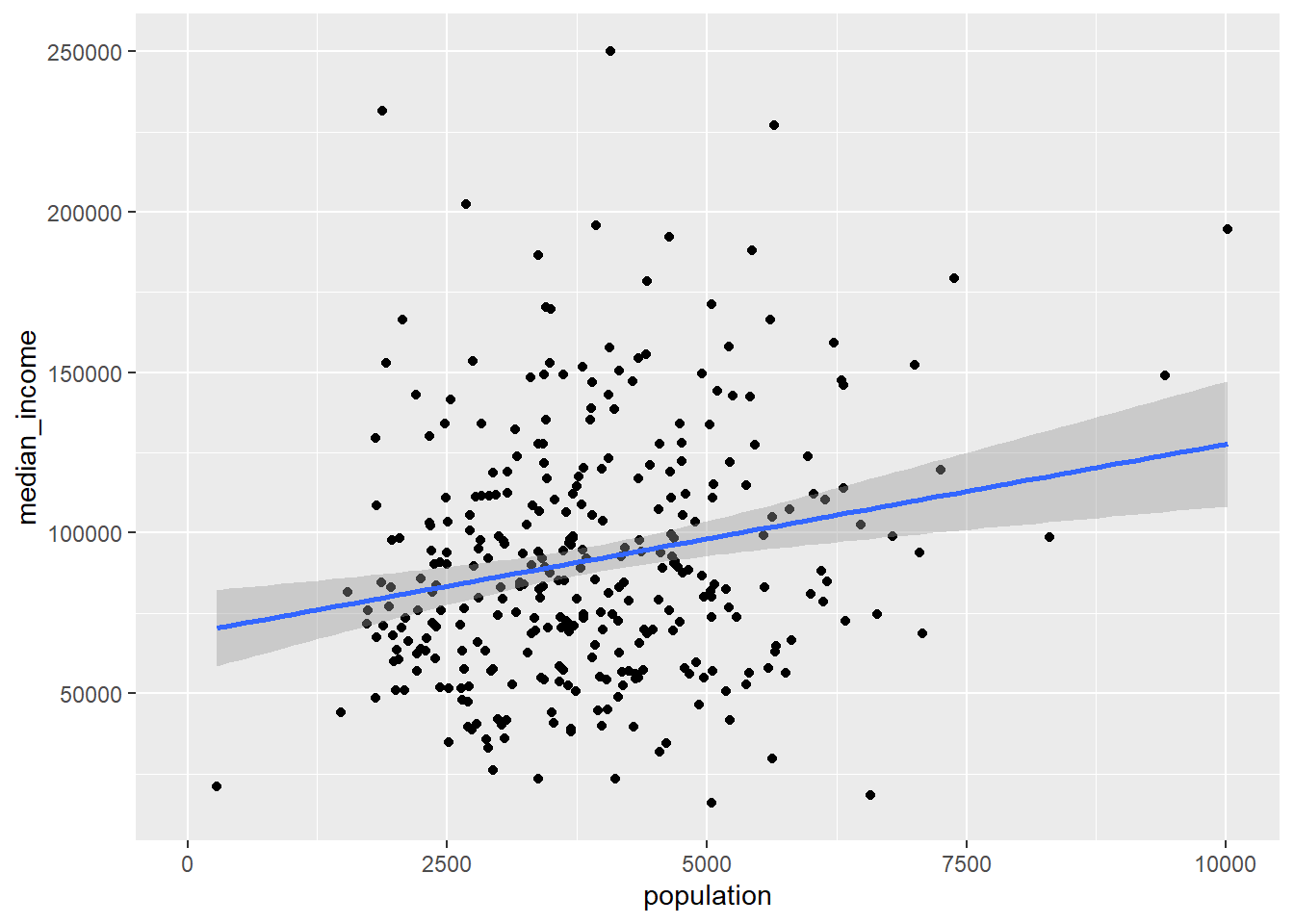

# Since census data comes with the geometry of census tracts, we can 
#   plot with geom_sf
ggplot(data = hennepin_tidycensus) + 
  geom_sf(aes(fill = median_income), colour = "white", linetype = 2) + 
  theme_void()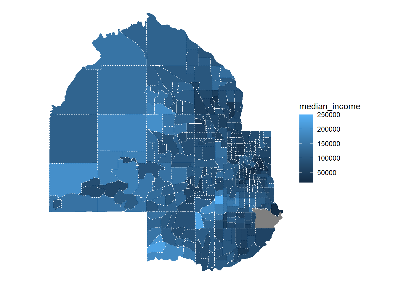

On Your Own - Census

Adapt the code in hennepin_tidycensus to write a function called MN_tract_data to give the user choices about year, county, and variables to pull off. Show that MN_tract_data(year = 2021, county = "Hennepin", variables = c("B01003_001", "B19013_001")) works as expected. Make sure it also works for other years, counties, and variables (e.g. B25077_001 is median home price and B02001_002 is number of white residents).
Use your function from (2) along with map and list_rbind to build a data set for Rice county for the years 2019-2021. Use your scraped data to plot trends in income over time and population over time.