You can download this .qmd file from here. Just hit the Download Raw File button.
Credit to Brianna Heggeseth and Leslie Myint from Macalester College for a few of these descriptions and examples.
Getting data from websites
Option 1: APIs
When we interact with sites like The New York Times, Zillow, and Google, we are accessing their data via a graphical layout (e.g., images, colors, columns) that is easy for humans to read but hard for computers.
An API stands for Application Programming Interface, and this term describes a general class of tool that allows computers, rather than humans, to interact with an organization’s data. How does this work?
When we use web browsers to navigate the web, our browsers communicate with web servers using a technology called HTTP or Hypertext Transfer Protocol to get information that is formatted into the display of a web page.
Programming languages such as R can also use HTTP to communicate with web servers. The easiest way to do this is via Web APIs, or Web Application Programming Interfaces, which focus on transmitting raw data, rather than images, colors, or other appearance-related information that humans interact with when viewing a web page.
A large variety of web APIs provide data accessible to programs written in R (and almost any other programming language!). Almost all reasonably large commercial websites offer APIs. Todd Motto has compiled an expansive list of Public Web APIs on GitHub, although it’s about 3 years old now so it’s not a perfect or complete list. Feel free to browse this list to see what data sources are available.
For our purposes of obtaining data, APIs exist where website developers make data nicely packaged for consumption. The language HTTP (hypertext transfer protocol) underlies APIs, and the R package httr() (and now the updated httr2()) was written to map closely to HTTP with R. Essentially you send a request to the website (server) where you want data from, and they send a response, which should contain the data (plus other stuff).
The case studies in this document provide a really quick introduction to data acquisition, just to get you started and show you what’s possible. For more information, these links can be somewhat helpful:
In R, it is easiest to use Web APIs through a wrapper package, an R package written specifically for a particular Web API.
The R development community has already contributed wrapper packages for many large Web APIs (e.g. ZillowR, rtweet, genius, Rspotify, tidycensus, etc.)
To find a wrapper package, search the web for “R package” and the name of the website. For example:
Searching for “R Weather.com package” returns weatherData
rOpenSci also has a good collection of wrapper packages.
In particular, tidycensus is a wrapper package that makes it easy to obtain desired census information for mapping and modeling:
Warning: • You have not set a Census API key. Users without a key are limited to 500
queries per day and may experience performance limitations.
ℹ For best results, get a Census API key at
http://api.census.gov/data/key_signup.html and then supply the key to the
`census_api_key()` function to use it throughout your tidycensus session.
This warning is displayed once per session.
Obtaining raw data from the Census Bureau was that easy! Often we will have to obtain and use a secret API key to access the data, but that’s not always necessary with tidycensus.
Now we can tidy that data and produce plots and analyses.
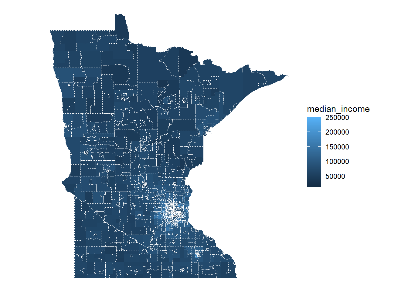
# Rename cryptic variables from the census formsample_acs_data <- sample_acs_data |>rename(population = B01003_001E,population_moe = B01003_001M,median_income = B19013_001E,median_income_moe = B19013_001M)# Plot with geom_sf since our data contains 1 row per census tract# with its geometryggplot(data = sample_acs_data) +geom_sf(aes(fill = median_income), colour ="white", linetype =2) +theme_void()
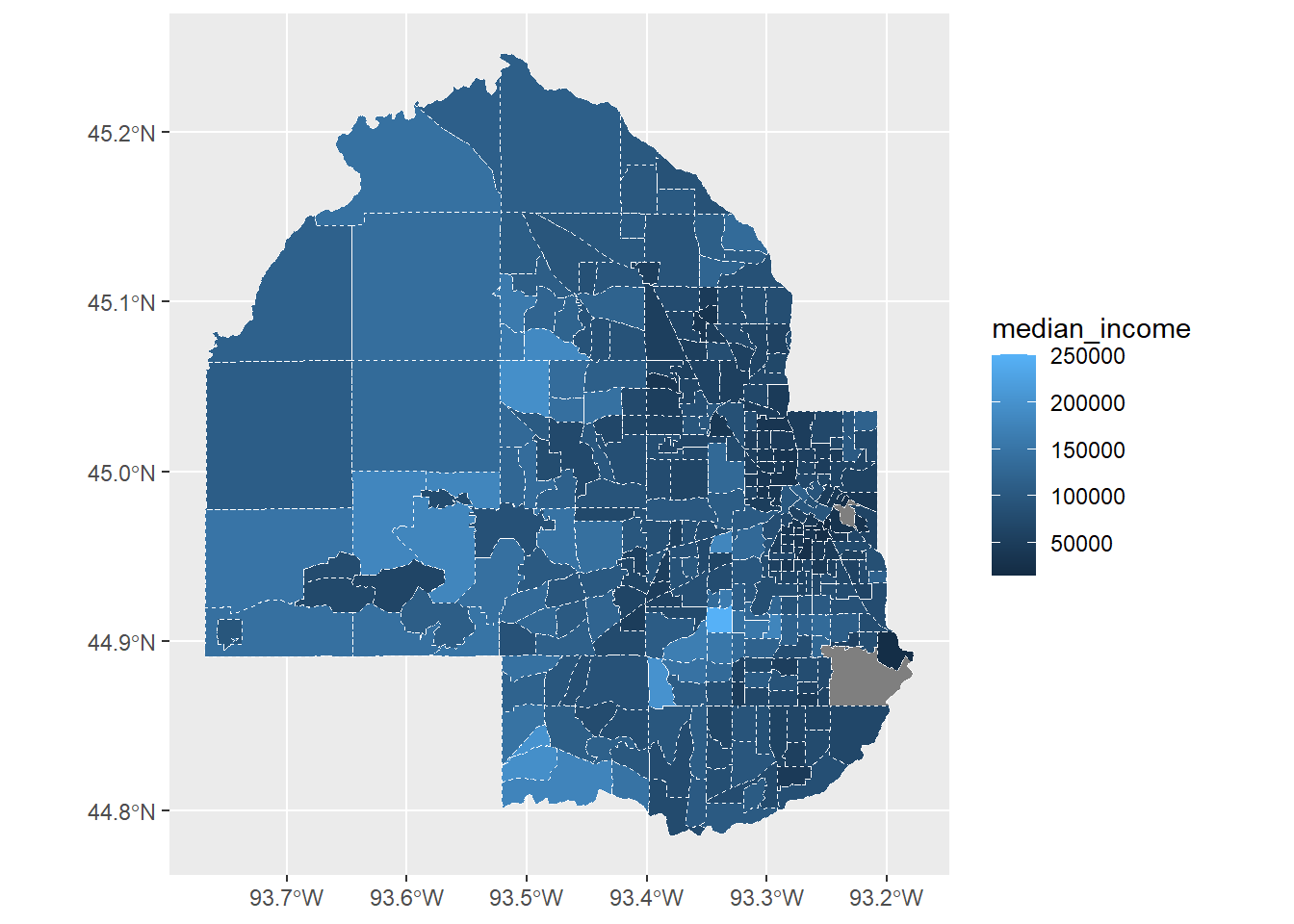
# The whole state of MN is overwhelming, so focus on a single countysample_acs_data |>filter(str_detect(NAME, "Hennepin")) |>ggplot() +geom_sf(aes(fill = median_income), colour ="white", linetype =2)
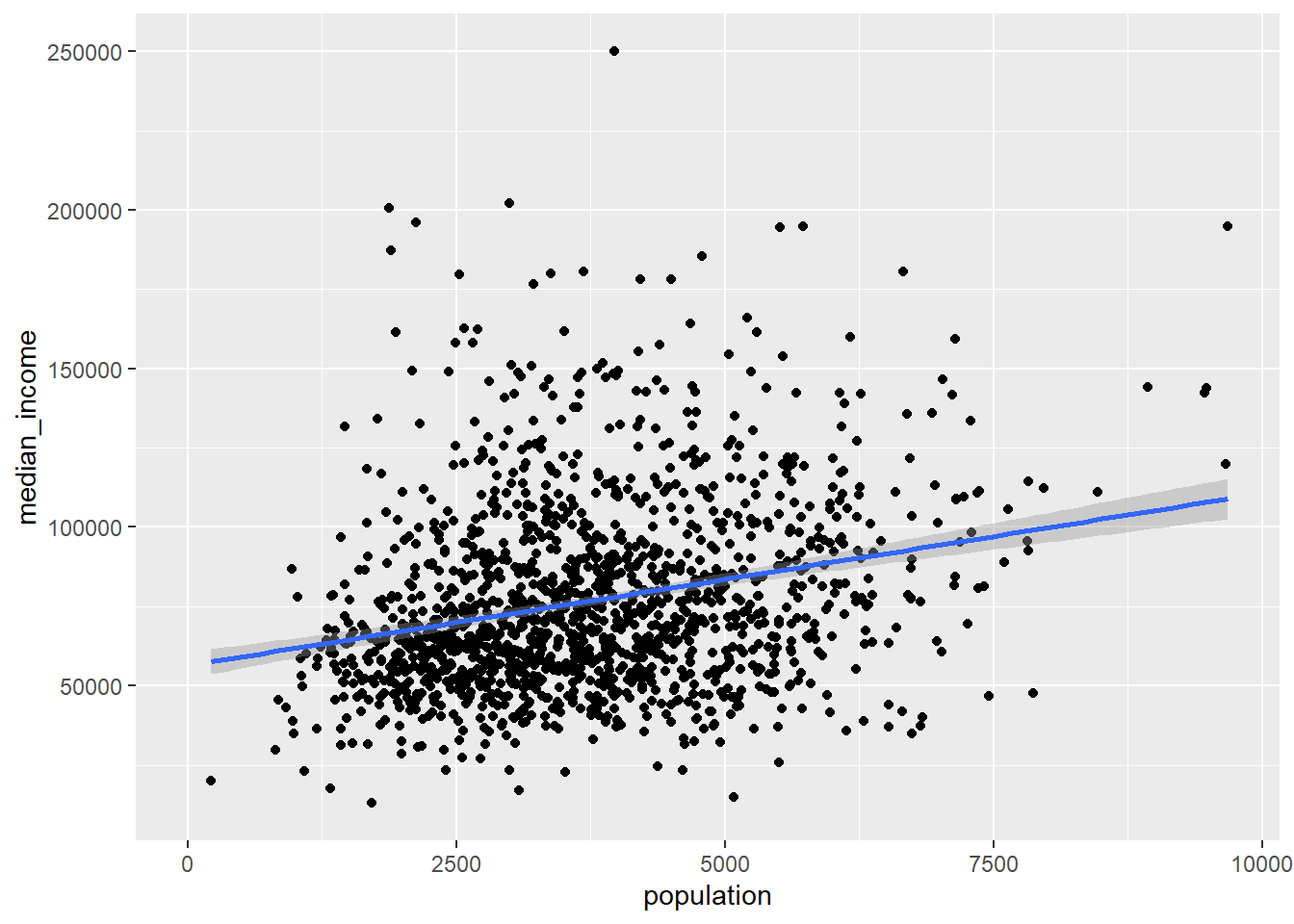
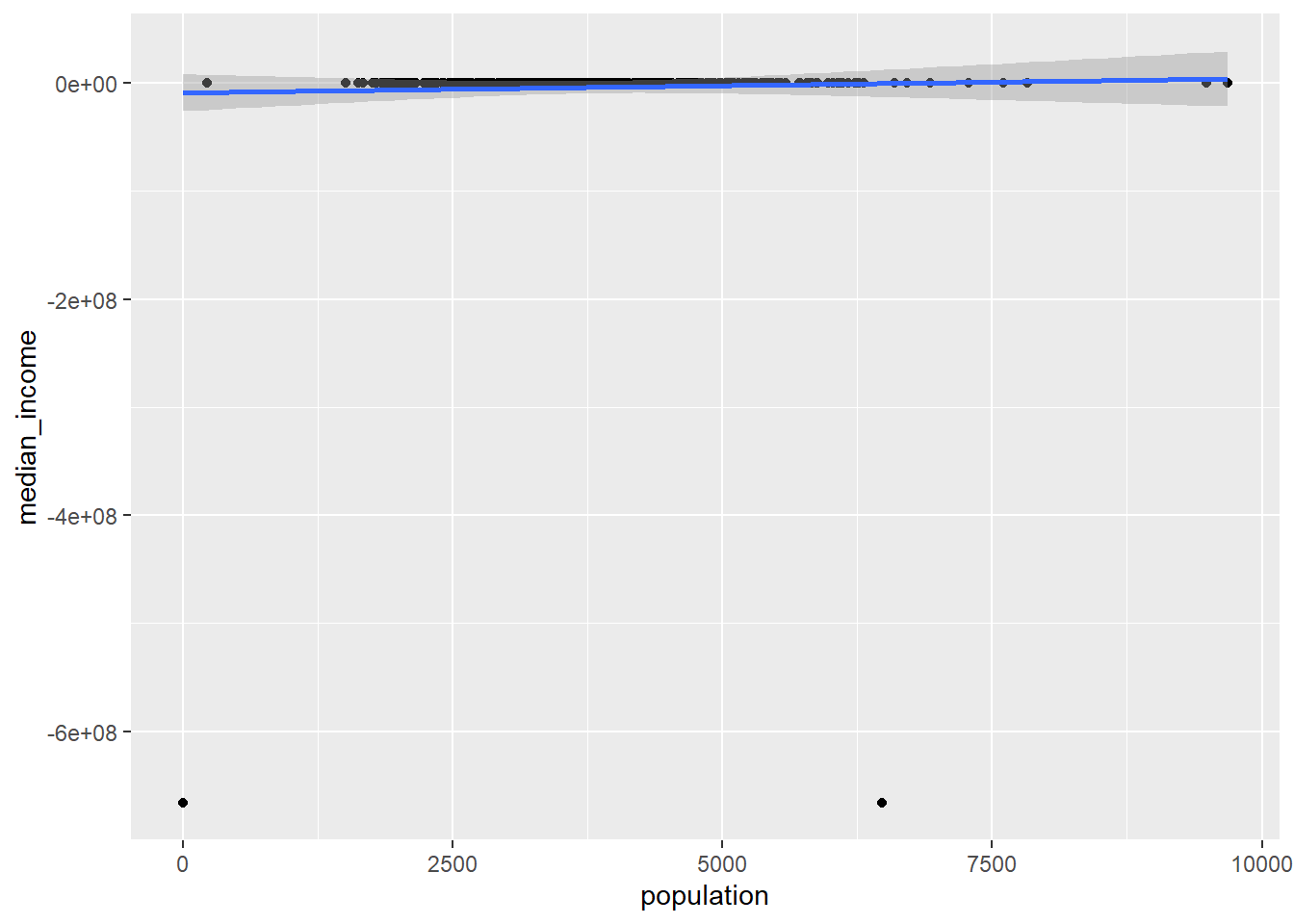
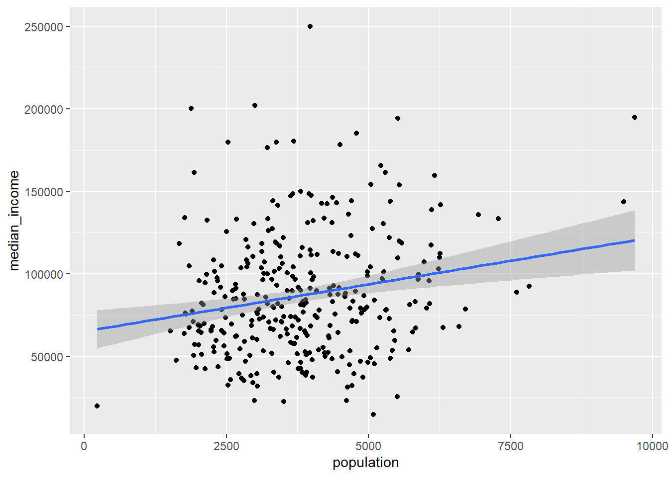
# Look for relationships between variables with 1 row per tractas_tibble(sample_acs_data) |>ggplot(aes(x = population, y = median_income)) +geom_point() +geom_smooth(method ="lm")
Extra resources:
tidycensus: wrapper package that provides an interface to a few census datasets with map geometry included!
get_acs() is one of the functions that is part of tidycensus. Let’s explore what’s going on behind the scenes with get_acs()…
Accessing web APIs directly
Getting a Census API key
Many APIs (and their wrapper packages) require users to obtain a key to use their services.
This lets organizations keep track of what data is being used.
It also rate limits their API and ensures programs don’t make too many requests per day/minute/hour. Be aware that most APIs do have rate limits — especially for their free tiers.
Your request for a new API key has been successfully submitted. Please check your email. In a few minutes you should receive a message with instructions on how to activate your new key.
Check your email. Copy and paste your key into a new text file:
File > New File > Text File (towards the bottom of the menu)
Save as census_api_key.txt in the same folder as this .qmd.
You could then read in the key with code like this:
While this works, the problem is once we start backing up our files to GitHub, your API key will also appear on GitHub, and you want to keep your API key secret. Thus, we might use environment variables instead:
One way to store a secret across sessions is with environment variables. Environment variables, or envvars for short, are a cross platform way of passing information to processes. For passing envvars to R, you can list name-value pairs in a file called .Renviron in your home directory. The easiest way to edit it is to run:
file.edit("~/.Renviron")
The file looks something like
PATH = “path” VAR1 = “value1” VAR2 = “value2” And you can access the values in R using Sys.getenv():
Sys.getenv("VAR1")#> [1] "value1"
Note that .Renviron is only processed on startup, so you’ll need to restart R to see changes.
Another option is to use Sys.setenv and Sys.getenv:
# I used the first line to store my CENSUS API key in .Renviron# after uncommenting - should only need to run one time# Sys.setenv("CENSUS_KEY" = "my census api key pasted here")# my_census_api_key <- Sys.getenv("CENSUS_KEY")
Let’s look at the Population Estimates Example and the American Community Survey (ACS) Example. These examples walk us through the steps to incrementally build up a URL to obtain desired data. This URL is known as a web API request.
http://: The scheme, which tells your browser or program how to communicate with the web server. This will typically be either http: or https:.
api.census.gov: The hostname, which is a name that identifies the web server that will process the request.
data/2019/acs/acs1: The path, which tells the web server how to get to the desired resource.
In the case of the Census API, this locates a desired dataset in a particular year.
Other APIs allow search functionality. (e.g., News organizations have article searches.) In these cases, the path locates the search function we would like to call.
?get=NAME,B02015_009E,B02015_009M&for=state:*: The query parameters, which provide the parameters for the function you would like to call.
We can view this as a string of key-value pairs separated by &. That is, the general structure of this part is key1=value1&key2=value2.
key
value
get
NAME,B02015_009E,B02015_009M
for
state:*
Typically, each of these URL components will be specified in the API documentation. Sometimes, the scheme, hostname, and path (https://api.census.gov/data/2019/acs/acs1) will be referred to as the endpoint for the API call.
We will first use the httr2 package to build up a full URL from its parts.
request() creates an API request object using the base URL
req_url_path_append() builds up the URL by adding path components separated by /
req_url_query() adds the ? separating the endpoint from the query and sets the key-value pairs in the query
The .multi argument controls how multiple values for a given key are combined.
The I() function around "state:*" inhibits parsing of special characters like : and *. (It’s known as the “as-is” function.)
The backticks around for are needed because for is a reserved word in R (for for-loops). You’ll need backticks whenever the key name has special characters (like spaces, dashes).
We can see from here that providing an API key is achieved with key=YOUR_API_KEY.
# Request total number of Hmong residents and margin of error by state# in 2019, as in the User GuideCENSUS_API_KEY <-Sys.getenv("CENSUS_API_KEY")req <-request("https://api.census.gov") |>req_url_path_append("data") |>req_url_path_append("2019") |>req_url_path_append("acs") |>req_url_path_append("acs1") |>req_url_query(get =c("NAME", "B02015_009E", "B02015_009M"), `for`=I("state:*"), key = CENSUS_API_KEY, .multi ="comma")
Why would we ever use these steps instead of just using the full URL as a string?
To generalize this code with functions! (This is exactly what wrapper packages do.)
To handle special characters
e.g., query parameters might have spaces, which need to be represented in a particular way in a URL (URLs can’t contain spaces)
Once we’ve fully constructed our request, we can use req_perform() to send out the API request and get a response.
resp <-req_perform(req)resp
We see from Content-Type that the format of the response is something called JSON. We can navigate to the request URL to see the structure of this output.
JSON (Javascript Object Notation) is a nested structure of key-value pairs.
We can use resp_body_json() to parse the JSON into a nicer format.
Without simplifyVector = TRUE, the JSON is read in as a list.
     NAME       B02015_009E B02015_009M state
[1,] "Illinois" "655"       "511"       "17"
[2,] "Georgia"  "3162"      "1336"      "13"
[3,] "Idaho"    NA          NA          "16"
[4,] "Hawaii"   "56"        "92"        "15"
[5,] "Indiana"  "1344"      "1198"      "18"
[6,] "Iowa"     "685"       "705"       "19"
All right, let’s try this! First we’ll grab total population and median household income for all census tracts in MN using 3 approaches
# First using tidycenuslibrary(tidycensus)sample_acs_data <- tidycensus::get_acs(year =2021,state ="MN",geography ="tract",variables =c("B01003_001", "B19013_001"),output ="wide",geometry =TRUE,county ="Hennepin", # specify county in callshow_call =TRUE# see resulting query)
Write a for loop to obtain the Hennepin County data from 2017-2021
Write a function to give choices about year, county, and variables
Use your function from (2) along with map and list_rbind to build a data set for Rice county for the years 2019-2021
One more example using an API key
Here’s an example of getting data from a website that attempts to make imdb movie data available as an API.
Initial instructions:
go to omdbapi.com under the API Key tab and request a free API key
store your key as discussed earlier
explore the examples at omdbapi.com
We will first obtain data about the movie Coco from 2017.
myapikey <-Sys.getenv("OMDB_KEY")# Find url exploring examples at omdbapi.comurl <-str_c("http://www.omdbapi.com/?t=Coco&y=2017&apikey=", myapikey)coco <-GET(url) # coco holds response from servercoco # Status of 200 is good!details <-content(coco, "parse") details # get a list of 25 pieces of informationdetails$Year # how to access detailsdetails[[2]] # since a list, another way to access
Now build a data set for a collection of movies
# Must figure out pattern in URL for obtaining different movies# - try searching for othersmovies <-c("Coco", "Wonder+Woman", "Get+Out", "The+Greatest+Showman", "Thor:+Ragnarok")# Set up empty tibbleomdb <-tibble(Title =character(), Rated =character(), Genre =character(),Actors =character(), Metascore =double(), imdbRating =double(),BoxOffice =double())# Use for loop to run through API request process 5 times,# each time filling the next row in the tibble# - can do max of 1000 GETs per dayfor(i in1:5) { url <-str_c("http://www.omdbapi.com/?t=",movies[i],"&apikey=", myapikey)Sys.sleep(0.5) onemovie <-GET(url) details <-content(onemovie, "parse") omdb[i,1] <- details$Title omdb[i,2] <- details$Rated omdb[i,3] <- details$Genre omdb[i,4] <- details$Actors omdb[i,5] <-parse_number(details$Metascore) omdb[i,6] <-parse_number(details$imdbRating) omdb[i,7] <-parse_number(details$BoxOffice) # no $ and ,'s}omdb# could use stringr functions to further organize this data - separate # different genres, different actors, etc.
On Your Own (continued)
(Based on final project by Mary Wu and Jenna Graff, MSCS 264, Spring 2024). Start with a small data set on 56 national parks from kaggle, and supplement with columns for the park address (a single column including address, city, state, and zip code) and a list of available activities (a single character column with activities separated by commas) from the park websites themselves.
Rows: 56 Columns: 6
── Column specification ────────────────────────────────────────────────────────
Delimiter: ","
chr (3): Park Code, Park Name, State
dbl (3): Acres, Latitude, Longitude

ℹ Use `spec()` to retrieve the full column specification for this data.
ℹ Specify the column types or set `show_col_types = FALSE` to quiet this message.