Table Scraping in R

You can download this .qmd file from here. Just hit the Download Raw File button.

Using rvest for web scraping

If you would like to assemble data from a website with no API, you can often acquire data using more brute force methods commonly called web scraping. Typically, this involves finding content inside HTML (Hypertext markup language) code used for creating webpages and web applications and the CSS (Cascading style sheets) language for customizing the appearance of webpages. We are used to reading data from .csv files…. but most websites have it stored in XML (like html, but for data). You can read more about it here if you’re interested: https://www.w3schools.com/xml/default.asp

XML has a sort of tree or graph-like structure… so we can identify information by which node it belongs to (html_nodes) and then convert the content into something we can use in R (html_text or html_table).

Here’s one quick example of web scraping. First check out the webpage https://www.cheese.com/by_type and then select Semi-Soft. We can drill into the html code for this webpage and find and store specific information (like cheese names)

session <- bow("https://www.cheese.com/by_type", force = TRUE)
result <- scrape(session, query=list(t="semi-soft", per_page=100)) |>
  html_node("#main-body") |> 
  html_nodes("h3") |> 
  html_text()
head(result)

[1] "American Cheese"     "Mozzarella"          "Taleggio"           
[4] "Fontina Val d'Aosta" "Blue Cheese"         "Jarlsberg"

#> [1] "3-Cheese Italian Blend"  "Abbaye de Citeaux"      
#> [3] "Abbaye du Mont des Cats" "Adelost"                
#> [5] "ADL Brick Cheese"        "Ailsa Craig"

Four steps to scraping data with functions in the `rvest` library:

robotstxt::paths_allowed() Check if the website allows scraping, and then make sure we scrape “politely”
read_html(). Input the URL containing the data and turn the html code into an XML file (another markup format that’s easier to work with).
html_nodes(). Extract specific nodes from the XML file by using the CSS path that leads to the content of interest. (use css=“table” for tables.)
html_text(). Extract content of interest from nodes. Might also use html_table() etc.

Data scraping ethics

Before scraping, we should always check first whether the website allows scraping. We should also consider if there’s any personal or confidential information, and we should be considerate to not overload the server we’re scraping from.

Chapter 24 in R4DS provides a nice overview of some of the important issues to consider. A couple of highlights:

be aware of terms of service, and, if available, the robots.txt file that some websites will publish to clarify what can and cannot be scraped and other constraints about scraping.
use the polite package to scrape public, non-personal, and factual data in a respectful manner
scrape with a good purpose and request only what you need; in particular, be extremely wary of personally identifiable information

See this article for more perspective on the ethics of data scraping.

When the data is already in table form:

In this example, we will scrape climate data from this website

The website already contains data in table form, so we use html_nodes(. , css = "table") and html_table()

# check that scraping is allowed (Step 0)
robotstxt::paths_allowed("https://www.usclimatedata.com/climate/minneapolis/minnesota/united-states/usmn0503")


 www.usclimatedata.com

[1] TRUE

# Step 1: read_html()
mpls <- read_html("https://www.usclimatedata.com/climate/minneapolis/minnesota/united-states/usmn0503")

# 2: html_nodes()
tables <- html_nodes(mpls, css = "table") 
tables  # have to guesstimate which table contains climate info

{xml_nodeset (8)}
[1] <table id="monthly_table_one" class="table table-hover tablesaw tablesaw- ...
[2] <table id="monthly_table_two" class="table table-hover tablesaw tablesaw- ...
[3] <table class="table table-hover tablesaw tablesaw-mode-swipe mt-4 daily_t ...
[4] <table class="table table-hover tablesaw tablesaw-mode-swipe mt-4 history ...
[5] <table class="table table-striped table-hover tablesaw tablesaw-mode-swip ...
[6] <table class="table table-hover tablesaw geo_table">\n<thead><tr>\n<th> < ...
[7] <table class="table table-hover tablesaw datetime_table" data-tablesaw-hi ...
[8] <table class="table table-hover tablesaw monthly_summary_table" data-tabl ...

# 3: html_table()
html_table(tables, header = TRUE, fill = TRUE)    # find the right table

[[1]]
# A tibble: 6 × 7
  ``                                    JanJa  FebFe  MarMa  AprAp  MayMa  JunJu
  <chr>                                 <dbl>  <dbl>  <dbl>  <dbl>  <dbl>  <dbl>
1 Average high in ºF Av. high Hi         24    29     41     58     69     79   
2 Average low in ºF Av. low Lo            8    13     24     37     49     59   
3 Days with precipitation Days precip.…   8     7     11      9     11     13   
4 Hours of sunshine Hours sun. Sun      140   166    200    231    272    302   
5 Av. precipitation in inch Av. precip…   0.9   0.77   1.89   2.66   3.36   4.25
6 Av. snowfall in inch Snowfall Sn       12     8     10      3      0      0   

[[2]]
# A tibble: 6 × 7
  ``                                     JulJu AugAu  SepSe  OctOc  NovNo  DecDe
  <chr>                                  <dbl> <dbl>  <dbl>  <dbl>  <dbl>  <dbl>
1 Average high in ºF Av. high Hi         83     80    72     58     41     27   
2 Average low in ºF Av. low Lo           64     62    52     40     26     12   
3 Days with precipitation Days precip.…  10     10     9      8      8      8   
4 Hours of sunshine Hours sun. Sun      343    296   237    193    115    112   
5 Av. precipitation in inch Av. precip…   4.04   4.3   3.08   2.43   1.77   1.16
6 Av. snowfall in inch Snowfall Sn        0      0     0      1      9     12   

[[3]]
# A tibble: 31 × 7
   Day    HighºF LowºF `Prec/moinch` `Prec/yrinch` `Snow/moinch` `Snow/yrinch`
   <chr>   <dbl> <dbl>         <dbl>         <dbl>         <dbl>         <dbl>
 1 1 Jan    23.8   8.3          0.04          0.04          0.39           1  
 2 2 Jan    23.7   8.2          0.08          0.08          0.71           1.8
 3 3 Jan    23.6   8.1          0.12          0.12          1.1            2.8
 4 4 Jan    23.5   7.9          0.12          0.12          1.5            3.8
 5 5 Jan    23.5   7.8          0.16          0.16          1.81           4.6
 6 6 Jan    23.4   7.7          0.2           0.2           2.2            5.6
 7 7 Jan    23.4   7.6          0.24          0.24          2.6            6.6
 8 8 Jan    23.3   7.5          0.28          0.28          3.11           7.9
 9 9 Jan    23.3   7.4          0.28          0.28          3.5            8.9
10 10 Jan   23.3   7.3          0.31          0.31          3.9            9.9
# ℹ 21 more rows

[[4]]
# A tibble: 26 × 6
   Day    HighºF LowºF Precip.inch Snowinch `Snow d.inch`
   <chr>   <dbl> <dbl> <chr>       <chr>            <dbl>
 1 01 Dec   32    19   0.07        1.61                 7
 2 02 Dec   27    12   0.00        0.00                 6
 3 03 Dec   37.9  19.9 0.00        0.00                 6
 4 04 Dec   39    24.1 0.00        0.00                 6
 5 05 Dec   37    21.9 0.00        0.00                 5
 6 06 Dec   32    17.1 0.00        0.00                 5
 7 07 Dec   42.1  21.9 0.00        0.00                 5
 8 08 Dec   41    30.9 0.00        0.00                 5
 9 09 Dec   34    -0.9 0.16        2.52                 5
10 10 Dec    8.1  -4   T           T                    7
# ℹ 16 more rows

[[5]]
# A tibble: 9 × 4
  ``                                          `Dec 19`    ``    Normal     
  <chr>                                       <chr>       <lgl> <chr>      
1 "Average high temperature Av. high temp."   "29.9 ºF"   NA    "27 ºF"    
2 "Average low temperature Av. low temp."     "14.6 ºF"   NA    "12 ºF"    
3 "Total precipitation Total precip."         "0.39 inch" NA    "1.16 inch"
4 "Total snowfall Total snowfall"             "6.33 inch" NA    "12 inch"  
5 ""                                          ""          NA    ""         
6 "Highest max temperature Highest max temp." "44.1 ºF"   NA    "-"        
7 "Lowest max temperature Lowest max temp."   "8.1 ºF"    NA    "-"        
8 "Highest min temperature Highest min temp." "32.0 ºF"   NA    "-"        
9 "Lowest min temperature Lowest min temp."   "-5.1 ºF"   NA    "-"        

[[6]]
# A tibble: 10 × 3
   ``                   ``                ``   
   <chr>                <chr>             <lgl>
 1 Country              United States     NA   
 2 State                Minnesota         NA   
 3 County               Hennepin          NA   
 4 City                 Minneapolis       NA   
 5 Zip code             55401             NA   
 6 Longitude            -93.27 dec. degr. NA   
 7 Latitude             44.98 dec. degr.  NA   
 8 Altitude - Elevation 840ft             NA   
 9 ICAO                 -                 NA   
10 IATA                 -                 NA   

[[7]]
# A tibble: 6 × 3
  ``          ``              ``   
  <chr>       <chr>           <lgl>
1 Local Time  10:19 PM        NA   
2 Sunrise     07:35 AM        NA   
3 Sunset      04:32 PM        NA   
4 Day / Night Night           NA   
5 Timezone    Chicago -6:00   NA   
6 Timezone DB America/Chicago NA   

[[8]]
# A tibble: 6 × 2
  ``                         ``        
  <chr>                      <chr>     
1 Annual high temperature    55ºF      
2 Annual low temperature     37ºF      
3 Days per year with precip. 112 days  
4 Annual hours of sunshine   2607 hours
5 Average annual precip.     30.61 inch
6 Av. annual snowfall        55 inch

mpls_data1 <- html_table(tables, header = TRUE, fill = TRUE)[[1]]  
mpls_data1

# A tibble: 6 × 7
  ``                                    JanJa  FebFe  MarMa  AprAp  MayMa  JunJu
  <chr>                                 <dbl>  <dbl>  <dbl>  <dbl>  <dbl>  <dbl>
1 Average high in ºF Av. high Hi         24    29     41     58     69     79   
2 Average low in ºF Av. low Lo            8    13     24     37     49     59   
3 Days with precipitation Days precip.…   8     7     11      9     11     13   
4 Hours of sunshine Hours sun. Sun      140   166    200    231    272    302   
5 Av. precipitation in inch Av. precip…   0.9   0.77   1.89   2.66   3.36   4.25
6 Av. snowfall in inch Snowfall Sn       12     8     10      3      0      0

mpls_data2 <- html_table(tables, header = TRUE, fill = TRUE)[[2]]  
mpls_data2

# A tibble: 6 × 7
  ``                                     JulJu AugAu  SepSe  OctOc  NovNo  DecDe
  <chr>                                  <dbl> <dbl>  <dbl>  <dbl>  <dbl>  <dbl>
1 Average high in ºF Av. high Hi         83     80    72     58     41     27   
2 Average low in ºF Av. low Lo           64     62    52     40     26     12   
3 Days with precipitation Days precip.…  10     10     9      8      8      8   
4 Hours of sunshine Hours sun. Sun      343    296   237    193    115    112   
5 Av. precipitation in inch Av. precip…   4.04   4.3   3.08   2.43   1.77   1.16
6 Av. snowfall in inch Snowfall Sn        0      0     0      1      9     12

Now we wrap the 4 steps above into the bow and scrape functions from the polite package:

session <- bow("https://www.usclimatedata.com/climate/minneapolis/minnesota/united-states/usmn0503", force = TRUE)

result <- scrape(session) |>
  html_nodes(css = "table") |> 
  html_table(header = TRUE, fill = TRUE)
mpls_data1 <- result[[1]]
mpls_data2 <- result[[2]]

Even after finding the correct tables, there may still be a lot of work to make it tidy!!!

[Pause to Ponder:] What is each line of code doing below?

bind_cols(mpls_data1, mpls_data2) |>
  as_tibble() |> 
  select(-`...8`) |>
  mutate(`...1` = str_extract(`...1`, "[^ ]+ [^ ]+ [^ ]+")) |>
  pivot_longer(cols = c(`JanJa`:`DecDe`), 
               names_to = "month", values_to = "weather") |>
  pivot_wider(names_from = `...1`, values_from = weather) |>
  mutate(month = str_sub(month, 1, 3))  |>
  rename(avg_high = "Average high in",
         avg_low = "Average low in")

New names:
• `` -> `...1`
• `` -> `...8`

# A tibble: 12 × 7
   month avg_high avg_low `Days with precipitation` `Hours of sunshine`
   <chr>    <dbl>   <dbl>                     <dbl>               <dbl>
 1 Jan         24       8                         8                 140
 2 Feb         29      13                         7                 166
 3 Mar         41      24                        11                 200
 4 Apr         58      37                         9                 231
 5 May         69      49                        11                 272
 6 Jun         79      59                        13                 302
 7 Jul         83      64                        10                 343
 8 Aug         80      62                        10                 296
 9 Sep         72      52                         9                 237
10 Oct         58      40                         8                 193
11 Nov         41      26                         8                 115
12 Dec         27      12                         8                 112
# ℹ 2 more variables: `Av. precipitation in` <dbl>, `Av. snowfall in` <dbl>

# Probably want to rename the rest of the variables too!

Leaflet mapping example with data in table form

Let’s return to our example from 02_maps.qmd where we recreated an interactive choropleth map of population densities by US state. Recall how that plot was very suspicious? The population density data that came with the state geometries from our source seemed incorrect.

Let’s see if we can use our new web scraping skills to scrape the correct population density data and repeat that plot! Can we go out and find the real statewise population densities, create a tidy data frame, merge that with our state geometry shapefiles, and then regenerate our plot?

A quick wikipedia search yields this webpage with more reasonable population densities in a nice table format. Let’s see if we can grab this data using our 4 steps to rvesting data!

# check that scraping is allowed (Step 0)
robotstxt::paths_allowed("https://en.wikipedia.org/wiki/List_of_states_and_territories_of_the_United_States_by_population_density")


 en.wikipedia.org

[1] TRUE

# Step 1: read_html()
pop_dens <- read_html("https://en.wikipedia.org/wiki/List_of_states_and_territories_of_the_United_States_by_population_density")

# 2: html_nodes()
tables <- html_nodes(pop_dens, css = "table") 
tables  # have to guesstimate which table contains our desired info

{xml_nodeset (2)}
[1] <table class="wikitable sortable plainrowheaders sticky-header-multi stat ...
[2] <table class="nowraplinks hlist mw-collapsible mw-collapsed navbox-inner" ...

# 3: html_table()
html_table(tables, header = TRUE, fill = TRUE)    # find the right table

[[1]]
# A tibble: 61 × 6
   Location               Density Density Population `Land area` `Land area`
   <chr>                  <chr>   <chr>   <chr>      <chr>       <chr>      
 1 Location               /mi2    /km2    Population mi2         km2        
 2 District of Columbia   11,131  4,297   678,972    61          158        
 3 New Jersey             1,263   488     9,290,841  7,354       19,047     
 4 Rhode Island           1,060   409     1,095,962  1,034       2,678      
 5 Puerto Rico            936     361     3,205,691  3,424       8,868      
 6 Massachusetts          898     347     7,001,399  7,800       20,202     
 7 Guam[4]                824     319     172,952    210         543        
 8 Connecticut            747     288     3,617,176  4,842       12,542     
 9 U.S. Virgin Islands[4] 737     284     98,750     134         348        
10 Maryland               637     246     6,180,253  9,707       25,142     
# ℹ 51 more rows

[[2]]
# A tibble: 11 × 2
   .mw-parser-output .navbar{display:inline;font-size:8…¹ .mw-parser-output .n…²
   <chr>                                                  <chr>                 
 1 "List of states and territories of the United States"  "List of states and t…
 2 "Demographics"                                         "Population\nAfrican …
 3 "Economy"                                              "Billionaires\nBudget…
 4 "Environment"                                          "Botanical gardens\nC…
 5 "Geography"                                            "Area\nBays\nBeaches\…
 6 "Government"                                           "Agriculture commissi…
 7 "Health"                                               "Changes in life expe…
 8 "History"                                              "Date of statehood\nN…
 9 "Law"                                                  "Abortion\nAge of con…
10 "Miscellaneous"                                        "Abbreviations\nAirpo…
11 "Category\n Commons\n Portals"                         "Category\n Commons\n…
# ℹ abbreviated names:
#   ¹`.mw-parser-output .navbar{display:inline;font-size:88%;font-weight:normal}.mw-parser-output .navbar-collapse{float:left;text-align:left}.mw-parser-output .navbar-boxtext{word-spacing:0}.mw-parser-output .navbar ul{display:inline-block;white-space:nowrap;line-height:inherit}.mw-parser-output .navbar-brackets::before{margin-right:-0.125em;content:"[ "}.mw-parser-output .navbar-brackets::after{margin-left:-0.125em;content:" ]"}.mw-parser-output .navbar li{word-spacing:-0.125em}.mw-parser-output .navbar a>span,.mw-parser-output .navbar a>abbr{text-decoration:inherit}.mw-parser-output .navbar-mini abbr{font-variant:small-caps;border-bottom:none;text-decoration:none;cursor:inherit}.mw-parser-output .navbar-ct-full{font-size:114%;margin:0 7em}.mw-parser-output .navbar-ct-mini{font-size:114%;margin:0 4em}html.skin-theme-clientpref-night .mw-parser-output .navbar li a abbr{color:var(--color-base)!important}@media(prefers-color-scheme:dark){html.skin-theme-clientpref-os .mw-parser-output .navbar li a abbr{color:var(--color-base)!important}}@media print{.mw-parser-output .navbar{display:none!important}}vteUnited States state-related lists`,
#   ²`.mw-parser-output .navbar{display:inline;font-size:88%;font-weight:normal}.mw-parser-output .navbar-collapse{float:left;text-align:left}.mw-parser-output .navbar-boxtext{word-spacing:0}.mw-parser-output .navbar ul{display:inline-block;white-space:nowrap;line-height:inherit}.mw-parser-output .navbar-brackets::before{margin-right:-0.125em;content:"[ "}.mw-parser-output .navbar-brackets::after{margin-left:-0.125em;content:" ]"}.mw-parser-output .navbar li{word-spacing:-0.125em}.mw-parser-output .navbar a>span,.mw-parser-output .navbar a>abbr{text-decoration:inherit}.mw-parser-output .navbar-mini abbr{font-variant:small-caps;border-bottom:none;text-decoration:none;cursor:inherit}.mw-parser-output .navbar-ct-full{font-size:114%;margin:0 7em}.mw-parser-output .navbar-ct-mini{font-size:114%;margin:0 4em}html.skin-theme-clientpref-night .mw-parser-output .navbar li a abbr{color:var(--color-base)!important}@media(prefers-color-scheme:dark){html.skin-theme-clientpref-os .mw-parser-output .navbar li a abbr{color:var(--color-base)!important}}@media print{.mw-parser-output .navbar{display:none!important}}vteUnited States state-related lists`

density_table <- html_table(tables, header = TRUE, fill = TRUE)[[1]]  
density_table

# A tibble: 61 × 6
   Location               Density Density Population `Land area` `Land area`
   <chr>                  <chr>   <chr>   <chr>      <chr>       <chr>      
 1 Location               /mi2    /km2    Population mi2         km2        
 2 District of Columbia   11,131  4,297   678,972    61          158        
 3 New Jersey             1,263   488     9,290,841  7,354       19,047     
 4 Rhode Island           1,060   409     1,095,962  1,034       2,678      
 5 Puerto Rico            936     361     3,205,691  3,424       8,868      
 6 Massachusetts          898     347     7,001,399  7,800       20,202     
 7 Guam[4]                824     319     172,952    210         543        
 8 Connecticut            747     288     3,617,176  4,842       12,542     
 9 U.S. Virgin Islands[4] 737     284     98,750     134         348        
10 Maryland               637     246     6,180,253  9,707       25,142     
# ℹ 51 more rows

# Perform Steps 0-3 using the polite package
session <- bow("https://en.wikipedia.org/wiki/List_of_states_and_territories_of_the_United_States_by_population_density", force = TRUE)

result <- scrape(session) |>
  html_nodes(css = "table") |> 
  html_table(header = TRUE, fill = TRUE)
density_table <- result[[1]]
density_table

# A tibble: 61 × 6
   Location               Density Density Population `Land area` `Land area`
   <chr>                  <chr>   <chr>   <chr>      <chr>       <chr>      
 1 Location               /mi2    /km2    Population mi2         km2        
 2 District of Columbia   11,131  4,297   678,972    61          158        
 3 New Jersey             1,263   488     9,290,841  7,354       19,047     
 4 Rhode Island           1,060   409     1,095,962  1,034       2,678      
 5 Puerto Rico            936     361     3,205,691  3,424       8,868      
 6 Massachusetts          898     347     7,001,399  7,800       20,202     
 7 Guam[4]                824     319     172,952    210         543        
 8 Connecticut            747     288     3,617,176  4,842       12,542     
 9 U.S. Virgin Islands[4] 737     284     98,750     134         348        
10 Maryland               637     246     6,180,253  9,707       25,142     
# ℹ 51 more rows

Even after grabbing our table from wikipedia and setting it in a nice tibble format, there is still some cleaning to do before we can merge this with our state geometries:

density_data <- density_table |>
  select(1, 2, 4, 5) |>
  filter(!row_number() == 1) |>
  rename(Land_area = `Land area`) |>
  mutate(state_name = str_to_lower(as.character(Location)),
         Density = parse_number(Density),
         Population = parse_number(Population),
         Land_area = parse_number(Land_area)) |>
  select(-Location)
density_data

# A tibble: 60 × 4
   Density Population Land_area state_name            
     <dbl>      <dbl>     <dbl> <chr>                 
 1   11131     678972        61 district of columbia  
 2    1263    9290841      7354 new jersey            
 3    1060    1095962      1034 rhode island          
 4     936    3205691      3424 puerto rico           
 5     898    7001399      7800 massachusetts         
 6     824     172952       210 guam[4]               
 7     747    3617176      4842 connecticut           
 8     737      98750       134 u.s. virgin islands[4]
 9     637    6180253      9707 maryland              
10     578      43915        76 american samoa[4]     
# ℹ 50 more rows

As before, we get core geometry data to draw US states and then we’ll make sure we can merge our new density data into the core files.

# Get info to draw US states for geom_polygon (connect the lat-long points)
states_polygon <- as_tibble(map_data("state")) |>
  select(region, group, order, lat, long)

# See what the state (region) levels look like in states_polygon
unique(states_polygon$region)

 [1] "alabama"              "arizona"              "arkansas"            
 [4] "california"           "colorado"             "connecticut"         
 [7] "delaware"             "district of columbia" "florida"             
[10] "georgia"              "idaho"                "illinois"            
[13] "indiana"              "iowa"                 "kansas"              
[16] "kentucky"             "louisiana"            "maine"               
[19] "maryland"             "massachusetts"        "michigan"            
[22] "minnesota"            "mississippi"          "missouri"            
[25] "montana"              "nebraska"             "nevada"              
[28] "new hampshire"        "new jersey"           "new mexico"          
[31] "new york"             "north carolina"       "north dakota"        
[34] "ohio"                 "oklahoma"             "oregon"              
[37] "pennsylvania"         "rhode island"         "south carolina"      
[40] "south dakota"         "tennessee"            "texas"               
[43] "utah"                 "vermont"              "virginia"            
[46] "washington"           "west virginia"        "wisconsin"           
[49] "wyoming"

# Get info to draw US states for geom_sf and leaflet (simple features
#   object with multipolygon geometry column)
states_sf <- read_sf("https://rstudio.github.io/leaflet/json/us-states.geojson") |>
  select(name, geometry)

# See what the state (name) levels look like in states_sf
unique(states_sf$name)

 [1] "Alabama"              "Alaska"               "Arizona"             
 [4] "Arkansas"             "California"           "Colorado"            
 [7] "Connecticut"          "Delaware"             "District of Columbia"
[10] "Florida"              "Georgia"              "Hawaii"              
[13] "Idaho"                "Illinois"             "Indiana"             
[16] "Iowa"                 "Kansas"               "Kentucky"            
[19] "Louisiana"            "Maine"                "Maryland"            
[22] "Massachusetts"        "Michigan"             "Minnesota"           
[25] "Mississippi"          "Missouri"             "Montana"             
[28] "Nebraska"             "Nevada"               "New Hampshire"       
[31] "New Jersey"           "New Mexico"           "New York"            
[34] "North Carolina"       "North Dakota"         "Ohio"                
[37] "Oklahoma"             "Oregon"               "Pennsylvania"        
[40] "Rhode Island"         "South Carolina"       "South Dakota"        
[43] "Tennessee"            "Texas"                "Utah"                
[46] "Vermont"              "Virginia"             "Washington"          
[49] "West Virginia"        "Wisconsin"            "Wyoming"             
[52] "Puerto Rico"

# See what the state (state_name) levels look like in density_data
unique(density_data$state_name)

 [1] "district of columbia"        "new jersey"                 
 [3] "rhode island"                "puerto rico"                
 [5] "massachusetts"               "guam[4]"                    
 [7] "connecticut"                 "u.s. virgin islands[4]"     
 [9] "maryland"                    "american samoa[4]"          
[11] "delaware"                    "florida"                    
[13] "new york"                    "pennsylvania"               
[15] "ohio"                        "northern mariana islands[4]"
[17] "california"                  "illinois"                   
[19] "hawaii"                      "north carolina"             
[21] "virginia"                    "georgia"                    
[23] "indiana"                     "south carolina"             
[25] "michigan"                    "tennessee"                  
[27] "new hampshire"               "washington"                 
[29] "texas"                       "kentucky"                   
[31] "wisconsin"                   "louisiana"                  
[33] "alabama"                     "missouri"                   
[35] "west virginia"               "minnesota"                  
[37] "vermont"                     "arizona"                    
[39] "mississippi"                 "oklahoma"                   
[41] "arkansas"                    "iowa"                       
[43] "colorado"                    "maine"                      
[45] "oregon"                      "utah"                       
[47] "kansas"                      "nevada"                     
[49] "nebraska"                    "idaho"                      
[51] "new mexico"                  "south dakota"               
[53] "north dakota"                "montana"                    
[55] "wyoming"                     "alaska"                     
[57] "contiguous us"               "50 states"                  
[59] "50 states and dc"            "united states"

# all lower case plus some extraneous rows

# Make sure all keys have the same format before joining: all lower case

states_sf <- states_sf |>
  mutate(name = str_to_lower(name))

# Now we can merge data sets together for the static and the interactive plots

# Merge with states_polygon (static)
density_polygon <- states_polygon |>
  left_join(density_data, by = c("region" = "state_name"))
density_polygon

# A tibble: 15,537 × 8
   region  group order   lat  long Density Population Land_area
   <chr>   <dbl> <int> <dbl> <dbl>   <dbl>      <dbl>     <dbl>
 1 alabama     1     1  30.4 -87.5     101    5108468     50645
 2 alabama     1     2  30.4 -87.5     101    5108468     50645
 3 alabama     1     3  30.4 -87.5     101    5108468     50645
 4 alabama     1     4  30.3 -87.5     101    5108468     50645
 5 alabama     1     5  30.3 -87.6     101    5108468     50645
 6 alabama     1     6  30.3 -87.6     101    5108468     50645
 7 alabama     1     7  30.3 -87.6     101    5108468     50645
 8 alabama     1     8  30.3 -87.6     101    5108468     50645
 9 alabama     1     9  30.3 -87.7     101    5108468     50645
10 alabama     1    10  30.3 -87.8     101    5108468     50645
# ℹ 15,527 more rows

# Looks like merge worked for 48 contiguous states plus DC
density_polygon |>
  group_by(region) |>
  summarise(mean = mean(Density)) |>
  print(n = Inf)

# A tibble: 49 × 2
   region                  mean
   <chr>                  <dbl>
 1 alabama                101  
 2 arizona                 65  
 3 arkansas                59  
 4 california             250  
 5 colorado                57  
 6 connecticut            747  
 7 delaware               529  
 8 district of columbia 11131  
 9 florida                422  
10 georgia                192  
11 idaho                   24  
12 illinois               226  
13 indiana                192  
14 iowa                    57  
15 kansas                  36  
16 kentucky               115  
17 louisiana              106  
18 maine                   45  
19 maryland               637  
20 massachusetts          898  
21 michigan               178  
22 minnesota               72  
23 mississippi             63  
24 missouri                90  
25 montana                  7.8
26 nebraska                26  
27 nevada                  29  
28 new hampshire          157  
29 new jersey            1263  
30 new mexico              17  
31 new york               415  
32 north carolina         223  
33 north dakota            11  
34 ohio                   288  
35 oklahoma                59  
36 oregon                  44  
37 pennsylvania           290  
38 rhode island          1060  
39 south carolina         179  
40 south dakota            12  
41 tennessee              173  
42 texas                  117  
43 utah                    42  
44 vermont                 70  
45 virginia               221  
46 washington             118  
47 west virginia           74  
48 wisconsin              109  
49 wyoming                  6

# Remove DC since such an outlier
density_polygon <- density_polygon |>
  filter(region != "district of columbia")


# Merge with states_sf (static or interactive)
density_sf <- states_sf |>
  left_join(density_data, by = c("name" = "state_name")) |>
  filter(!(name %in% c("alaska", "hawaii")))

# Looks like merge worked for 48 contiguous states plus DC and PR
class(density_sf)

[1] "sf"         "tbl_df"     "tbl"        "data.frame"

print(density_sf, n = Inf)

Simple feature collection with 50 features and 4 fields
Geometry type: MULTIPOLYGON
Dimension:     XY
Bounding box:  xmin: -124.7066 ymin: 17.92956 xmax: -65.6268 ymax: 49.38362
Geodetic CRS:  WGS 84
# A tibble: 50 × 5
   name                                    geometry Density Population Land_area
 * <chr>                         <MULTIPOLYGON [°]>   <dbl>      <dbl>     <dbl>
 1 alabama              (((-87.3593 35.00118, -85.…   101      5108468     50645
 2 arizona              (((-109.0425 37.00026, -10…    65      7431344    113594
 3 arkansas             (((-94.47384 36.50186, -90…    59      3067732     52035
 4 california           (((-123.2333 42.00619, -12…   250     38965193    155779
 5 colorado             (((-107.9197 41.00391, -10…    57      5877610    103642
 6 connecticut          (((-73.05353 42.03905, -71…   747      3617176      4842
 7 delaware             (((-75.41409 39.80446, -75…   529      1031890      1949
 8 district of columbia (((-77.03526 38.99387, -76… 11131       678972        61
 9 florida              (((-85.49714 30.99754, -85…   422     22610726     53625
10 georgia              (((-83.10919 35.00118, -83…   192     11029227     57513
11 idaho                (((-116.0475 49.00024, -11…    24      1964726     82643
12 illinois             (((-90.63998 42.51006, -88…   226     12549689     55519
13 indiana              (((-85.99006 41.75972, -84…   192      6862199     35826
14 iowa                 (((-91.36842 43.50139, -91…    57      3207004     55857
15 kansas               (((-101.906 40.00163, -95.…    36      2940546     81759
16 kentucky             (((-83.90335 38.76931, -83…   115      4526154     39486
17 louisiana            (((-93.60849 33.01853, -91…   106      4573749     43204
18 maine                (((-70.70392 43.05776, -70…    45      1395722     30843
19 maryland             (((-75.99465 37.95325, -76…   637      6180253      9707
20 massachusetts        (((-70.91752 42.88797, -70…   898      7001399      7800
21 michigan             (((-83.45424 41.73234, -84…   178     10037261     56539
22 minnesota            (((-92.0147 46.7054, -92.0…    72      5737915     79627
23 mississippi          (((-88.47111 34.9957, -88.…    63      2939690     46923
24 missouri             (((-91.83396 40.60957, -91…    90      6196156     68742
25 montana              (((-104.0475 49.00024, -10…     7.8    1132812    145546
26 nebraska             (((-103.3246 43.00299, -10…    26      1978379     76824
27 nevada               (((-117.0279 42.00071, -11…    29      3194176    109781
28 new hampshire        (((-71.08183 45.3033, -71.…   157      1402054      8953
29 new jersey           (((-74.23655 41.14083, -73…  1263      9290841      7354
30 new mexico           (((-107.4213 37.00026, -10…    17      2114371    121298
31 new york             (((-73.34381 45.01303, -73…   415     19571216     47126
32 north carolina       (((-80.97866 36.56211, -80…   223     10835491     48618
33 north dakota         (((-97.22874 49.00024, -97…    11       783926     69001
34 ohio                 (((-80.5186 41.9788, -80.5…   288     11785935     40861
35 oklahoma             (((-100.0877 37.00026, -94…    59      4053824     68595
36 oregon               (((-123.2113 46.17414, -12…    44      4233358     95988
37 pennsylvania         (((-79.76278 42.25265, -79…   290     12961683     44743
38 rhode island         (((-71.19684 41.67757, -71…  1060      1095962      1034
39 south carolina       (((-82.76414 35.0669, -82.…   179      5373555     30061
40 south dakota         (((-104.0475 45.94411, -96…    12       919318     75811
41 tennessee            (((-88.05487 36.49638, -88…   173      7126489     41235
42 texas                (((-101.8129 36.50186, -10…   117     30503301    261232
43 utah                 (((-112.1644 41.99523, -11…    42      3417734     82170
44 vermont              (((-71.50355 45.01303, -71…    70       647464      9217
45 virginia             (((-75.39766 38.0135, -75.…   221      8715698     39490
46 washington           (((-117.0334 49.00024, -11…   118      7812880     66456
47 west virginia        (((-80.5186 40.63695, -80.…    74      1770071     24038
48 wisconsin            (((-90.41543 46.56848, -90…   109      5910955     54158
49 wyoming              (((-109.0808 45.00207, -10…     6       584057     97093
50 puerto rico          (((-66.44834 17.98433, -66…   936      3205691      3424

# Remove DC and PR
density_sf <- density_sf |>
  filter(name != "district of columbia" & name != "puerto rico")

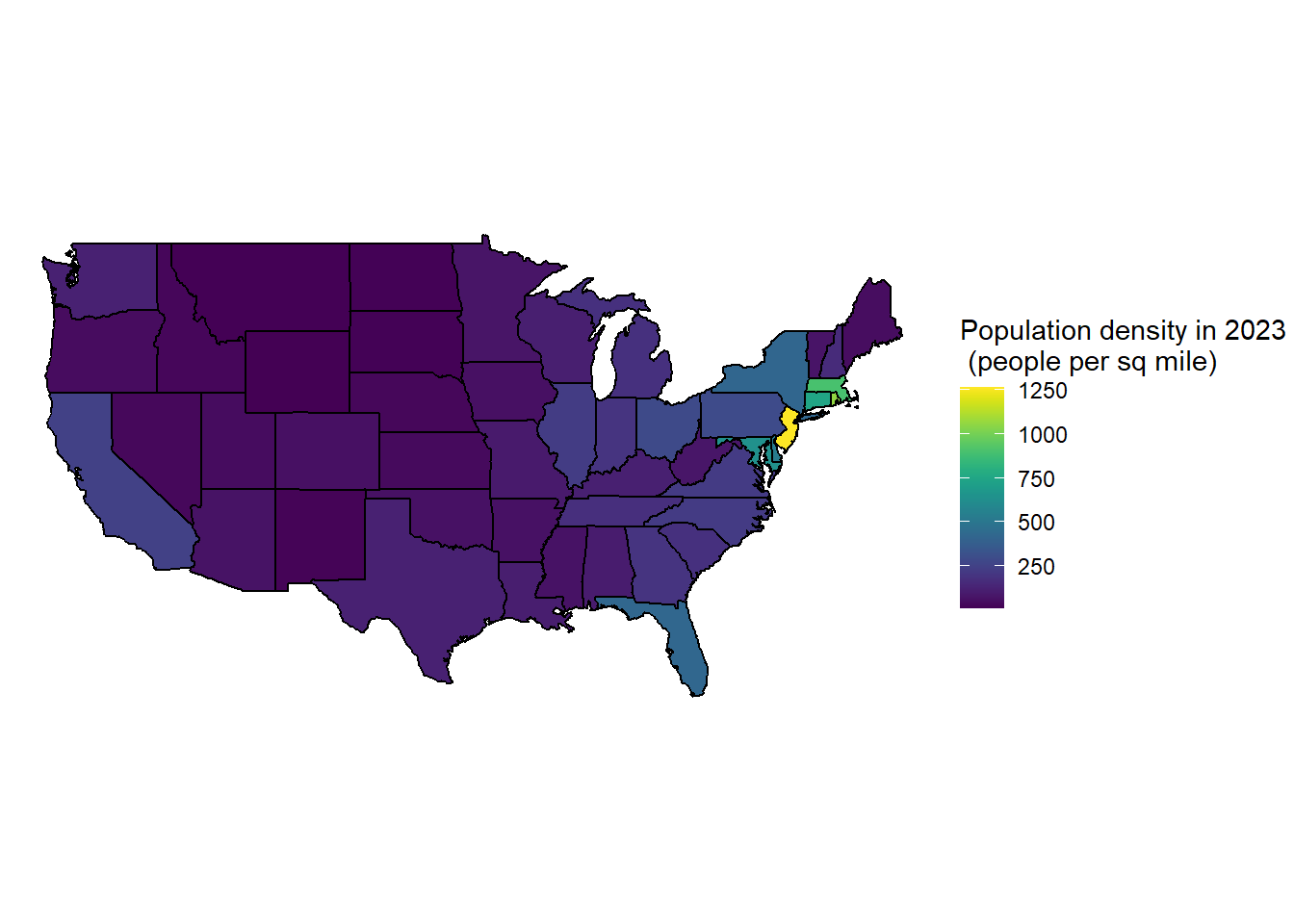
Numeric variable (static plot):

density_polygon |>
  ggplot(mapping = aes(x = long, y = lat, group = group)) + 
    geom_polygon(aes(fill = Density), color = "black") + 
    labs(fill = "Population density in 2023 \n (people per sq mile)") +
    coord_map() + 
    theme_void() +  
    scale_fill_viridis()

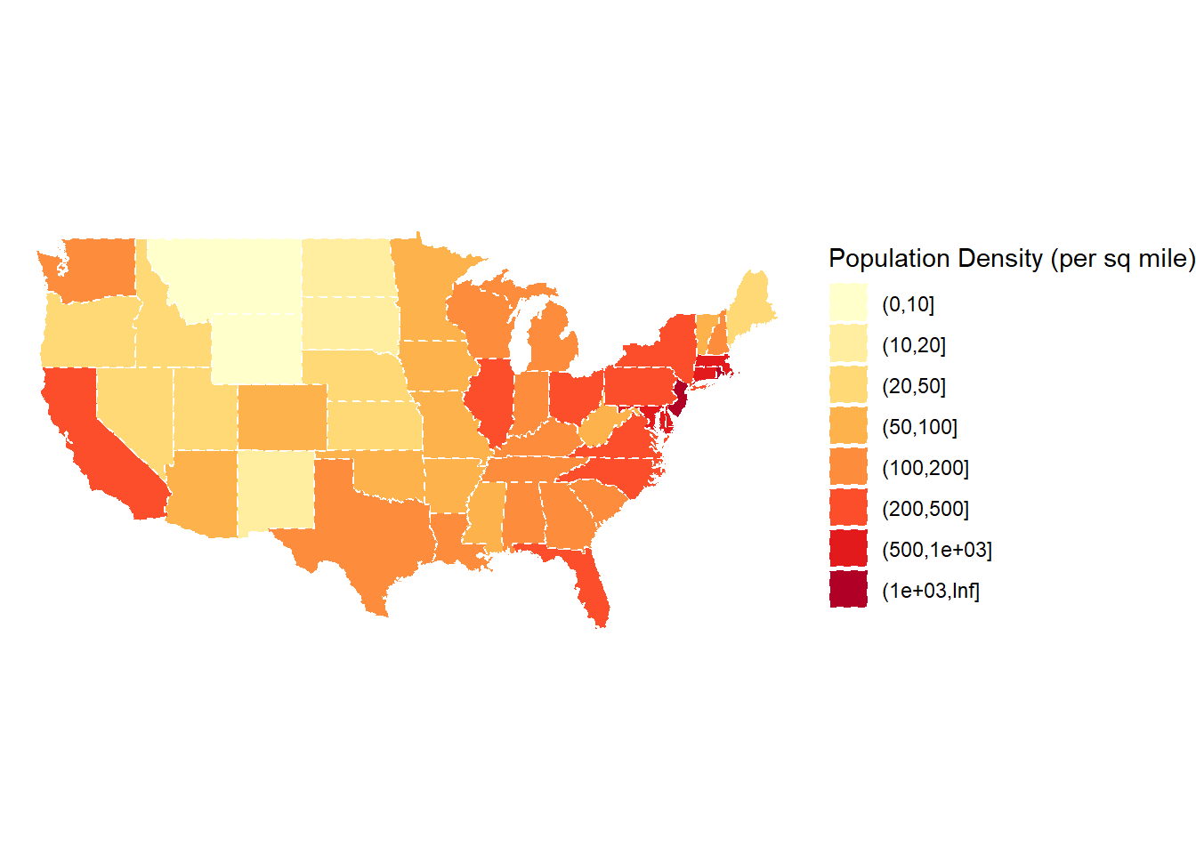
Remember that the original plot classified densities into our own pre-determined bins before plotting - this might look better!

density_polygon <- density_polygon |>
  mutate(Density_intervals = cut(Density, n = 8,
          breaks = c(0, 10, 20, 50, 100, 200, 500, 1000, Inf)))

density_polygon |>
  ggplot(mapping = aes(x = long, y = lat, group = group)) + 
    geom_polygon(aes(fill = Density_intervals), color = "white",
                 linetype = 2) + 
    labs(fill = "Population Density (per sq mile)") +
    coord_map() + 
    theme_void() +  
    scale_fill_brewer(palette = "YlOrRd")

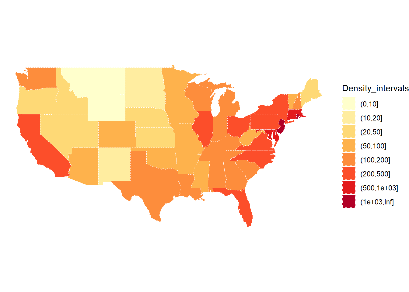
We could even create a static plot using geom_sf() using density_sf:

density_sf <- density_sf |>
  mutate(Density_intervals = cut(Density, n = 8,
          breaks = c(0, 10, 20, 50, 100, 200, 500, 1000, Inf))) 

ggplot(data = density_sf) + 
  geom_sf(aes(fill = Density_intervals), colour = "white", linetype = 2) + 
  theme_void() +  
  scale_fill_brewer(palette = "YlOrRd")

But… why not make an interactive plot instead?

density_sf <- density_sf |>
  mutate(labels = str_c(name, ": ", Density, " people per sq mile in 2023"))

labels <- lapply(density_sf$labels, HTML)
pal <- colorNumeric("YlOrRd", density_sf$Density)

leaflet(density_sf) |>
  setView(-96, 37.8, 4) |>
  addTiles() |>
  addPolygons(
    weight = 2,
    opacity = 1,
    color = ~ pal(density_sf$Density),
    dashArray = "3",
    fillOpacity = 0.7,
    highlightOptions = highlightOptions(
      weight = 5,
      color = "#666",
      dashArray = "",
      fillOpacity = 0.7,
      bringToFront = TRUE),
    label = labels,
    labelOptions = labelOptions(
      style = list("font-weight" = "normal", padding = "3px 8px"),
      textsize = "15px",
      direction = "auto"))

# should use addLegend() but not trivial without pre-set bins

Here’s an interactive plot with our own bins:

# Create our own category bins for population densities
#   and assign the yellow-orange-red color palette
bins <- c(0, 10, 20, 50, 100, 200, 500, 1000, Inf)
pal <- colorBin("YlOrRd", domain = density_sf$Density, bins = bins)

# Create labels that pop up when we hover over a state.  The labels must
#   be part of a list where each entry is tagged as HTML code.
density_sf <- density_sf |>
  mutate(labels = str_c(name, ": ", Density, " people / sq mile"))
labels <- lapply(density_sf$labels, HTML)

# If want more HTML formatting, use these lines instead of those above:
# states <- states |>
#   mutate(labels = glue("<strong>{name}</strong><br/>{density} people / 
#   mi<sup>2</sup>"))
# labels <- lapply(states$labels, HTML)

leaflet(density_sf) |>
  setView(-96, 37.8, 4) |>
  addTiles() |>
  addPolygons(
    fillColor = ~pal(Density),
    weight = 2,
    opacity = 1,
    color = "white",
    dashArray = "3",
    fillOpacity = 0.7,
    highlightOptions = highlightOptions(
      weight = 5,
      color = "#666",
      dashArray = "",
      fillOpacity = 0.7,
      bringToFront = TRUE),
    label = labels,
    labelOptions = labelOptions(
      style = list("font-weight" = "normal", padding = "3px 8px"),
      textsize = "15px",
      direction = "auto")) |>
  addLegend(pal = pal, values = ~Density, opacity = 0.7, title = NULL,
    position = "bottomright")

On Your Own

Use the rvest package and html_table to read in the table of data found at the link here and create a scatterplot of land area versus the 2022 estimated population. I give you some starter code below; fill in the “???” and be sure you can explain what EVERY line of code does and why it’s necessary.

city_pop <- read_html("https://en.wikipedia.org/wiki/List_of_United_States_cities_by_population")

pop <- html_nodes(???, ???)
html_table(pop, header = TRUE, fill = TRUE)  # find right table
pop2 <- html_table(pop, header = TRUE, fill = TRUE)[[???]]
pop2

# perform the steps above with the polite package
session <- bow("https://en.wikipedia.org/wiki/List_of_United_States_cities_by_population", force = TRUE)

result <- scrape(session) |>
  html_nodes(???) |>
  html_table(header = TRUE, fill = TRUE)
pop2 <- result[[???]]
pop2

pop3 <- as_tibble(pop2[,c(1:6,8)]) |>
  slice(???) |>
  rename(`State` = `ST`,
         `Estimate2023` = `2023estimate`,
         `Census` = `2020census`,
         `Area` = `2020 land area`,
         `Density` = `2020 density`) |>
  mutate(Estimate2023 = parse_number(Estimate2023),
         Census = parse_number(Census),
         Change = ???   # get rid of % but preserve +/-,
         Area = parse_number(Area),
         Density = parse_number(Density)) |> 
  mutate(City = str_replace(City, "\\[.*$", ""))
pop3

# pick out unusual points
outliers <- pop3 |> 
  filter(Estimate2023 > ??? | Area > ???)

# This will work if don't turn variables from chr to dbl, but in that 
#  case notice how axes are just evenly spaced categorical variables
ggplot(pop3, aes(x = ???, y = ???)) +
  geom_point()  +
  geom_smooth() +
  ggrepel::geom_label_repel(data = ???, aes(label = ???))

We would like to create a tibble with 4 years of data (2001-2004) from the Minnesota Wild hockey team. Specifically, we are interested in the “Scoring Regular Season” table from this webpage and the similar webpages from 2002, 2003, and 2004. Your final tibble should have 6 columns: player, year, age, pos (position), gp (games played), and pts (points).

You should (a) write a function called hockey_stats with inputs for team and year to scrape data from the “scoring Regular Season” table, and (b) use iteration techniques to scrape and combine 4 years worth of data. Here are some functions you might consider:

row_to_names(row_number = 1) from the janitor package
clean_names() also from the janitor package
bow() and scrape() from the polite package
str_c() from the stringr package (for creating urls with user inputs)
map2() and list_rbind() for iterating and combining years

Try following these steps:

Be sure you can find and clean the correct table from the 2021 season.
Organize your rvest code from (1) into functions from the polite package.
Place the code from (2) into a function where the user can input a team and year. You would then adjust the url accordingly and produce a clean table for the user.
Use map2 and list_rbind to build one data set containing Minnesota Wild data from 2001-2004.